Integrated trading strategy

In this tutorial, you will learn:

• How to make use of different features to write a strategy
• How to use machine learning models to predict trading signals

Putting it all together

In this part we’ll look into how to put everything together in order to build a strategy that incorporates different features (technical indicator, macroeconomic trends and sentiment indicator) so as to comprehensively examine the market as a whole.

Simple approach

We’ll first look into simplistic, rule-based methods to make use of the features in an algorithmic trading pipeline.

Baseline model

We have created the Baseline model example to demonstrate how we could generate signals using a technical analysis strategy, then filter it by macroeconomic data and sentiment labels. The implementation of the baseline model could be found in integrated-strategy/baseline.py.

The workflow of the baseline model is as follows:

• Generate the signals dataframe using a technical analysis strategy (e.g. MACD)
• Pass the signals to the macroeconomic filter
• Pass the signals to the sentiment filter
• Backtest with the filtered signals dataframe

As usual, we first select the ticker and time range to run the strategy:

# load price data
df_whole = pd.read_csv('../../database/microeconomic_data/hkex_ticks_day/hkex_0001.csv', header=0, index_col='Date', parse_dates=True)

ticker = "0005.HK"

# select time range (for trading)
start_date = pd.Timestamp('2017-01-01')
end_date = pd.Timestamp('2021-01-01')

df = df_whole.loc[start_date:end_date]

Note that we’ll also need this filered_df additionally to calculate the stock price’s sensitivity to economic indicators.

# get filtered df for macro analysis
filtered_df = df_whole.loc[:end_date]

In the example, we choose to apply the MACD crossover strategy.

# apply MACD crossover strategy
macd_cross = macdCrossover(df)
macd_fig = macd_cross.plot_MACD()
plt.close() # hide figure

# get signals dataframe
signals = macd_cross.gen_signals()
print(signals.head())
signal_fig = macd_cross.plot_signals(signals)
plt.close()  # hide figure

After obtaining the signals dataframe by running the technical analysis strategy, we’ll pass it to the macroeconomic filters and sentiment filter to eliminate signals that are contradicatory with the economic indicator or sentiment labels.

In this code snippet, we first apply the macroeconomic filter:

# get ticker's sensitivity to macro data
s_gdp, s_unemploy, s_property = GetSensitivity(filtered_df)

# append signals with macro data
signals = GetMacrodata(signals)

# calculate adjusting factor
signals['macro_factor'] = s_gdp * signals['GDP'] + s_unemploy * signals['Unemployment rate'] + s_property * signals['Property price']
signals['signal'] = signals['signal'] + signals['macro_factor']

# round off signals['signal'] to the nearest integer
signals['signal'] = signals['signal'].round(0)

We then apply the sentiment filter:

filtered_signals = SentimentFilter(ticker, signals)

With this filtered signals dataframe, we could pass it directly to the backtesting function in order to evaluate the portfolio performance.

portfolio, backtest_fig = Backtest(ticker, filtered_signals, df)
plt.close() # hide figure

# print stats
print("Final total value: {value:.4f} ".format(value=portfolio['total'][-1]))
print("Total return: {value:.4f}%".format(value=(((portfolio['total'][-1] - portfolio['total'][0])/portfolio['total'][-1]) * 100))) # for analysis
print("No. of trade: {value}".format(value=len(signals[signals.positions == 1])))

We could also make use of the evaluation metric functions:

# Evaluate strategy

# 1. Portfolio return
returns_fig = PortfolioReturn(portfolio)
returns_fig.suptitle('Baseline - Portfolio return')
#returns_fig.savefig('./figures/baseline_portfolo-return')
plt.show()

# 2. Sharpe ratio
sharpe_ratio = SharpeRatio(portfolio)
print("Sharpe ratio: {ratio:.4f} ".format(ratio = sharpe_ratio))

# 3. Maximum drawdown
maxDrawdown_fig, max_daily_drawdown, daily_drawdown = MaxDrawdown(df)
maxDrawdown_fig.suptitle('Baseline - Maximum drawdown', fontsize=14)
#maxDrawdown_fig.savefig('./figures/baseline_maximum-drawdown')
plt.show()

# 4. Compound Annual Growth Rate
cagr = CAGR(portfolio)
print("CAGR: {cagr:.4f} ".format(cagr = cagr))

Machine learning approach

Moving on, we’ll look into more advanced methods that pass the data features into a machine learning model in order to make sequential predictions.

Recurrent Neural Networks

A recurrent neural network (RNN) is a type of artificial neural network designed for sequential data or time series data. As opposed to traditional feedforward neural networks, they are networks with loops in them which allow information to persist. It has a lot of applications, ranging from language modelling to speech recognition. You can read more about the it in Andrej Karpathy’s blog post - The Unreasonable Effectiveness of Recurrent Neural Networks.

However, one problem with RNNs is that they have a hard time in capturing long-term dependencies. When making a prediction at the current time step, RNNs would weigh more recent historical information to be more important. But sometimes contextual information could lie in the far past. This is When LSTM comes into play.

The internal structure of an LSTM. [1]

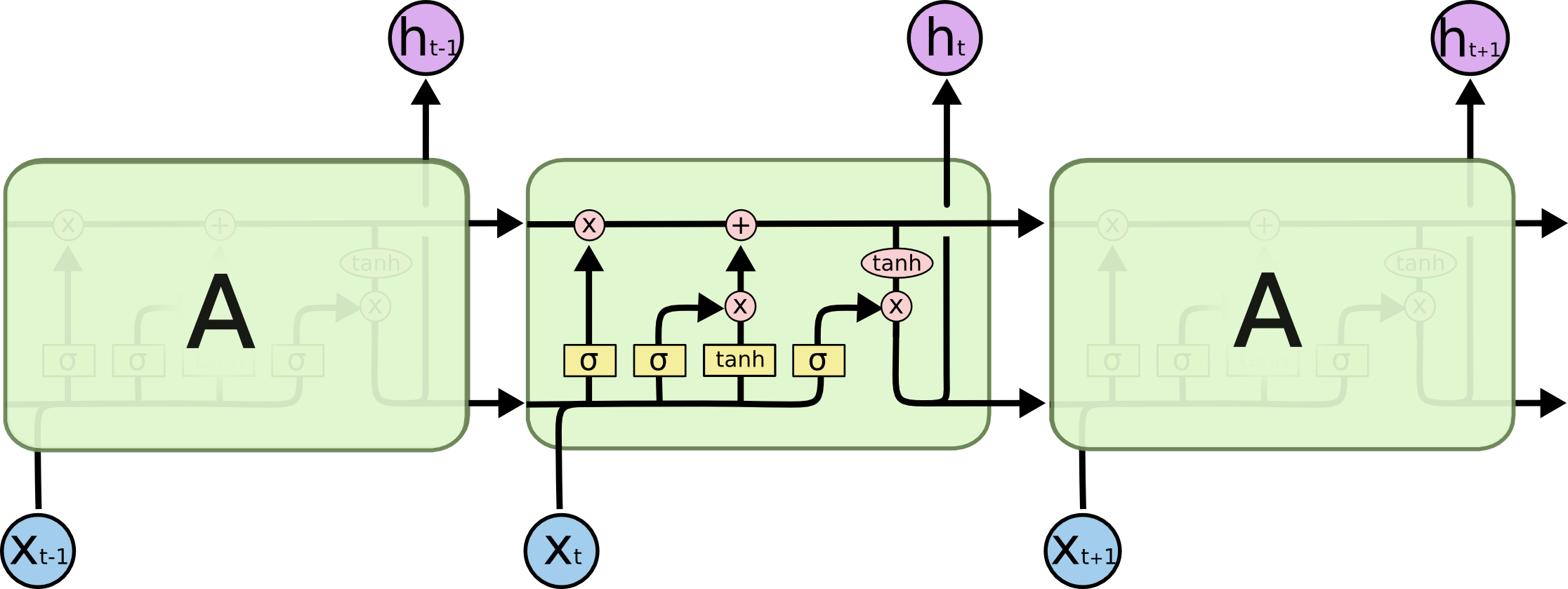
Long Short Term Memory networks (LSTMs) is an improved version of RNN that is specifically designed to avoid the long-term dependency problem. Their default behaviour is to remember information for long periods of time.

If you want to know more about the mechanism and details of LSTMs, you could read this great blog post - Understanding LSTM Networks.

Single-feature LSTM model

The implememtation of the single-feature LSTM model could be found in integrated-strategy/LSTM-train_price-only.py.

We’ll make use of the PyTorch library to build the LSTM model. You could install the library from here: https://pytorch.org/.

We first load the data for training and testing respectively.

data_dir = "../../database/microeconomic_data/hkex_ticks_day/"

# select date range
dates = pd.date_range('2010-01-02','2016-12-31',freq='B')
test_dates = pd.date_range('2017-01-03','2020-09-30',freq='B')

# select ticker
symbol = "0001"

# load data
df = read_data(data_dir, symbol, dates)
df_test = read_data(data_dir, symbol, test_dates)

The MinMaxScaler function from the sklearn.preprocessing is used to normalise the input features, i.e. they will be transformed into the range [-1,1] in the following code snippet.

scaler = MinMaxScaler(feature_range=(-1, 1))

df['Close'] = scaler.fit_transform(df['Close'].values.reshape(-1,1))
df_test['Close'] = scaler.fit_transform(df_test['Close'].values.reshape(-1,1))

look_back = 60 # choose sequence length

We can check the shapes of the train and test data:

x_train, y_train, x_test, y_test = load_data(df, look_back)
print('x_train.shape = ',x_train.shape)
print('y_train.shape = ',y_train.shape)
print('x_test.shape = ',x_test.shape)
print('y_test.shape = ',y_test.shape)

And then make the traing and testing sets in torch:

# make training and test sets in torch
x_train = torch.from_numpy(x_train).type(torch.Tensor)
x_test = torch.from_numpy(x_test).type(torch.Tensor)
y_train = torch.from_numpy(y_train).type(torch.Tensor)
y_test = torch.from_numpy(y_test).type(torch.Tensor)

Moving on, let’s set the hyperparameters.

# Hyperparameters
n_steps = look_back - 1
batch_size = 32
num_epochs = 100
input_dim = 1
hidden_dim = 32
num_layers = 2
output_dim = 1
torch.manual_seed(1) # set seed

We’ll use mean squared error (MSE) as the loss function, and use Adam as the optimiser with a learning rate of 0.01.

train = torch.utils.data.TensorDataset(x_train,y_train)
test = torch.utils.data.TensorDataset(x_test,y_test)

train_loader = torch.utils.data.DataLoader(dataset=train,
                                          batch_size=batch_size,
                                          shuffle=False)

test_loader = torch.utils.data.DataLoader(dataset=test,
                                          batch_size=batch_size,
                                          shuffle=False)



model = LSTM(input_dim=input_dim, hidden_dim=hidden_dim, output_dim=output_dim, num_layers=num_layers)

loss_fn = torch.nn.MSELoss()
optimiser = torch.optim.Adam(model.parameters(), lr=0.01)

We’ll write the training loop now:

# Initialise a list to store the losses
hist = np.zeros(num_epochs)

# Number of steps to unroll
seq_dim = look_back - 1

# Train model
for t in range(num_epochs):
    # Forward pass
    y_train_pred = model(x_train)
    loss = loss_fn(y_train_pred, y_train)

    if t % 10 == 0 and t !=0:
        print("Epoch ", t, "MSE: ", loss.item())

    hist[t] = loss.item()

    # Zero out gradient, else they will accumulate between epochs
    optimiser.zero_grad()

    # Backward pass
    loss.backward()

    # Update parameters
    optimiser.step()

We could now make predictions on the test set to get the MSE:

# Make predictions
y_test_pred = model(x_test)

# Invert predictions
y_train_pred = scaler.inverse_transform(y_train_pred.detach().numpy())
y_train = scaler.inverse_transform(y_train.detach().numpy())
y_test_pred = scaler.inverse_transform(y_test_pred.detach().numpy())
y_test = scaler.inverse_transform(y_test.detach().numpy())

# Calculate root mean squared error
trainScore = math.sqrt(mean_squared_error(y_train[:,0], y_train_pred[:,0]))
print('Train Score: %.2f RMSE' % (trainScore))
testScore = math.sqrt(mean_squared_error(y_test[:,0], y_test_pred[:,0]))
print('Test Score: %.2f RMSE' % (testScore))

Eventually, we’ll carry out inferencing and save the output signals dataframe for backtesting:

# Inferencing
y_inf_pred, y_inf = predict_price(df_test, model, scaler)
signal = gen_signal(y_inf_pred, y_inf)

# Save signals as csv file
output_df = pd.DataFrame(index=df_test.index)
output_df['signal'] = signal
output_df.index.name = "Date"

output_filename = 'output/' + symbol + '_output.csv'
output_df.to_csv(output_filename)

With the signals csv files, we could simply run output-backtester_wrapper.py in the same directory that would load all the files in the output directory and run it with the backtester_wrapper to compute the evaluation metrics.

Multi-feature LSTM model

The implememtation of the single-feature LSTM model could be found in integrated-strategy/LSTM-train_wrapper.py.

We’ll focus on looking at the LSTM_predict function, as the main function is simply a wrapper that calls the LSTM_predict function with different ticker symbols.

The code structure of the multi-feature LSTM and single-feature LSTM is largely the name, except that we’ll need the merged dataframe as the input and we’ll need to change the input/output dimensions of the model.

# load file
dir_name = os.getcwd()
data_dir = os.path.join(dir_name,"database_real/machine_learning_data/")
sentiment_data_dir=os.path.join(dir_name,"database/sentiment_data/data-result/")

# Get merged df with stock tick and sentiment scores
df, scaled, scaler = merge_data(symbol, data_dir, sentiment_data_dir, strategy)

look_back = 60 # choose sequence length

x_train, y_train, x_test_df, y_test_df = load_data(scaled, look_back)

# make training and test sets in torch
x_train = torch.from_numpy(x_train).type(torch.Tensor)
x_test = torch.from_numpy(x_test_df).type(torch.Tensor)
y_train = torch.from_numpy(y_train).type(torch.Tensor)
y_test = torch.from_numpy(y_test_df).type(torch.Tensor)

# Hyperparameters
num_epochs = 100
lr = 0.01
batch_size = 72
input_dim = 7
hidden_dim = 64
num_layers = 4
output_dim = 7
torch.manual_seed(1) # set seed

print("Hyperparameters:")
print("input_dim: ", input_dim, ", hidden_dim: ", hidden_dim, ", num_layers: ", num_layers, ", output_dim", output_dim)
print("num_epochs: ", num_epochs, ", batch_size: ", batch_size, ", lr: ", lr)

train = torch.utils.data.TensorDataset(x_train,y_train)
test = torch.utils.data.TensorDataset(x_test,y_test)

train_loader = torch.utils.data.DataLoader(dataset=train,
                                      batch_size=batch_size,
                                      shuffle=False)

test_loader = torch.utils.data.DataLoader(dataset=test,
                                      batch_size=batch_size,
                                      shuffle=False)

model = LSTM(input_dim=input_dim, hidden_dim=hidden_dim, output_dim=output_dim, num_layers=num_layers)

loss_fn = torch.nn.MSELoss()
optimiser = torch.optim.Adam(model.parameters(), lr=lr)

hist = np.zeros(num_epochs)

# Number of steps to unroll
seq_dim = look_back - 1

# Train model
for t in range(num_epochs):
    for i, (train_data, train_label) in enumerate(train_loader):
        # Forward pass
        train_pred = model(train_data)
        loss = loss_fn(train_pred, train_label)

        hist[t] = loss.item()

        # Zero out gradient, else they will accumulate between epochs
        optimiser.zero_grad()

        # Backward pass
        loss.backward()

        # Update parameters
        optimiser.step()

    if t % 10 == 0 and t != 0:
        y_train_pred = model(x_train)
        loss = loss_fn(y_train_pred, y_train)
        print("Epoch ", t, "MSE: ", loss.item())

# Make predictions
y_test_pred = model(x_test)

# Invert predictions
y_train_pred = scaler.inverse_transform(y_train_pred.detach().numpy())
y_train = scaler.inverse_transform(y_train.detach().numpy())
y_test_pred = scaler.inverse_transform(y_test_pred.detach().numpy())
y_test = scaler.inverse_transform(y_test.detach().numpy())

# Calculate root mean squared error
trainScore = math.sqrt(mean_squared_error(y_train[:,0], y_train_pred[:,0]))
print('Train Score: %.2f RMSE' % (trainScore))
testScore = math.sqrt(mean_squared_error(y_test[:,0], y_test_pred[:,0]))
print('Test Score: %.2f RMSE' % (testScore))

visualise(df, y_test[:,0], y_test_pred[:,0], pred_filename)

signal_dataframe = gen_signal(y_test_pred[:,0], y_test[:,0], df[len(df)-len(y_test):].index, by_trend=True)

# Save signals as csv file
output_filename = 'LSTM_output_trend/' + symbol + '_output.csv'
signal_dataframe.to_csv(output_filename,index=False)

Note that we’ll need to pass the ticker symbol name and the name of the technical indicator (to be included in the merged dataframe) to the LSTM_predict function, for example by calling in this way:

LSTM_predict('0001', 'macd-crossover')

Similarly, we could run the output-backtester_wrapper.py file to backtest the output signals.

References

• Long Short Term Memory

Image sources

[1]	By Christopher Olah - Understanding LSTM Networks, https://colah.github.io/posts/2015-08-Understanding-LSTMs

Attention

All investments entail inherent risk. This repository seeks to solely educate people on methodologies to build and evaluate algorithmic trading strategies. All final investment decisions are yours and as a result you could make or lose money.